4. Direct and Inverse Kinematics
Given the pose representation developed in the previous chapter, this chapter addresses the forward problem (computing end-effector pose from joint variables) and the inverse problem (finding joint variables that realise a desired end-effector pose). Both problems are central to robot programming: the controller works in joint space, but tasks are naturally specified in task space, so we need reliable maps in both directions.
1 The direct kinematics map
For a manipulator with joint variables \(\boldsymbol q\), the pose of the end-effector frame relative to the base is
\[ \mathbf{T}^b_e(\boldsymbol q) = \begin{bmatrix} \hat{\boldsymbol n}^b_e & \hat{\boldsymbol s}^b_e & \hat{\boldsymbol a}^b_e & \boldsymbol{p}^b_e\\ 0 & 0 & 0 & 1 \end{bmatrix} = \begin{bmatrix} \mathbf{R}& \boldsymbol{p}^b_e\\ \mathbf 0^{\mathsf{T}}& 1 \end{bmatrix}, \]
where \((\hat{\boldsymbol n},\hat{\boldsymbol s},\hat{\boldsymbol a})\) are the end-effector frame unit vectors and \(\boldsymbol{p}^b_e\) is its origin. An open chain with \(n\) joints decomposes this into a product of link transforms:
\[ \mathbf{T}^0_n(\boldsymbol q) = \mathbf{A}^0_1(q_1)\,\mathbf{A}^1_2(q_2)\cdots\mathbf{A}^{n-1}_n(q_n), \]
and including fixed base and tool offsets,
\[ \mathbf{T}^b_e = \mathbf{T}^b_0\;\mathbf{T}^0_n(\boldsymbol q)\;\mathbf{T}^n_e . \]
Joint space and task space. The joint configuration \(\boldsymbol q \in \mathbb{R}^n\) lives in joint space. The end-effector pose \(\boldsymbol x \in \mathbb{R}^m\) (position + orientation) lives in task space. The map \(\boldsymbol x = h(\boldsymbol q)\) is in general nonlinear, which makes the inverse problem non-trivial.
1.1 Worked example: two-link planar arm
For a planar arm with link lengths \(a_1,a_2\) and joint angles \(\theta_1,\theta_2\), write \(c_1=\cos\theta_1\), \(c_{12}=\cos(\theta_1+\theta_2)\), etc. The end-effector transform is
\[ \mathbf{T}^b_e(\theta_1,\theta_2) = \begin{bmatrix} 0 & s_{12} & c_{12} & a_1 c_1 + a_2 c_{12}\\ 0 & -c_{12} & s_{12} & a_1 s_1 + a_2 s_{12}\\ 1 & 0 & 0 & 0\\ 0 & 0 & 0 & 1 \end{bmatrix}. \]
The position entries make geometric sense: the end-effector reach is the vector sum of two link vectors projected onto \(x\) and \(y\).
For longer kinematic chains a systematic, rule-based approach is essential.
2 The Denavit–Hartenberg convention
The Denavit–Hartenberg (DH) convention attaches a frame to each link using exactly four parameters per joint. It provides the systematic, rule-based approach that makes analysis of longer kinematic chains tractable. A worked animation of the frame-assignment procedure is available on ILIAS.
| Parameter | Symbol | Description |
|---|---|---|
| Link length | \(a_i\) | distance between \(z_{i-1}\) and \(z_i\) along \(x_i\) |
| Link twist | \(\alpha_i\) | angle between \(z_{i-1}\) and \(z_i\) about \(x_i\) |
| Link offset | \(d_i\) | distance between \(x_{i-1}\) and \(x_i\) along \(z_{i-1}\) |
| Joint angle | \(\theta_i\) | angle between \(x_{i-1}\) and \(x_i\) about \(z_{i-1}\) |
Frame assignment rules:
- Choose axis \(z_i\) along the axis of joint \(i+1\).
- Locate origin \(O_i\) at the intersection of \(z_i\) with the common normal to \(z_{i-1}\) and \(z_i\).
- Choose \(x_i\) along the common normal from joint \(i\) to joint \(i+1\).
- Choose \(y_i\) to complete a right-handed frame.
For a revolute joint, \(\theta_i\) is the variable and \(d_i\) is fixed. For a prismatic joint, \(d_i\) is the variable and \(\theta_i\) is fixed.
2.1 DH link transform
The transform from frame \(i-1\) to frame \(i\) factors into a screw along \(z\) and a screw along \(x\):
\[ \mathbf{A}^{i-1}_{i'} = \begin{bmatrix} c_{\theta_i} & -s_{\theta_i} & 0 & 0\\ s_{\theta_i} & c_{\theta_i} & 0 & 0\\ 0 & 0 & 1 & d_i\\ 0 & 0 & 0 & 1 \end{bmatrix}, \qquad \mathbf{A}^{i'}_{i} = \begin{bmatrix} 1 & 0 & 0 & a_i\\ 0 & c_{\alpha_i} & -s_{\alpha_i} & 0\\ 0 & s_{\alpha_i} & c_{\alpha_i} & 0\\ 0 & 0 & 0 & 1 \end{bmatrix}. \]
Their product is the standard DH link matrix:
\[ \mathbf{A}^{i-1}_i = \begin{bmatrix} c_{\theta_i} & -s_{\theta_i}c_{\alpha_i} & s_{\theta_i}s_{\alpha_i} & a_i c_{\theta_i}\\ s_{\theta_i} & c_{\theta_i}c_{\alpha_i} & -c_{\theta_i}s_{\alpha_i} & a_i s_{\theta_i}\\ 0 & s_{\alpha_i} & c_{\alpha_i} & d_i\\ 0 & 0 & 0 & 1 \end{bmatrix}. \]
3 DH examples
3.1 Three-link planar arm (3R)
All joints revolute, all axes parallel to \(z\), all twists \(\alpha_i = 0\).
| Link | \(a_i\) | \(\alpha_i\) | \(d_i\) | \(\theta_i\) |
|---|---|---|---|---|
| 1 | \(a_1\) | \(0\) | \(0\) | \(\theta_1^*\) |
| 2 | \(a_2\) | \(0\) | \(0\) | \(\theta_2^*\) |
| 3 | \(a_3\) | \(0\) | \(0\) | \(\theta_3^*\) |
With all twists zero the chain stays planar. Using \(c_{123}=\cos(\theta_1+\theta_2+\theta_3)\),
\[ \mathbf{T}^0_3 = \mathbf{A}^0_1\mathbf{A}^1_2\mathbf{A}^2_3 = \begin{bmatrix} c_{123} & -s_{123} & 0 & a_1 c_1 + a_2 c_{12} + a_3 c_{123}\\ s_{123} & c_{123} & 0 & a_1 s_1 + a_2 s_{12} + a_3 s_{123}\\ 0 & 0 & 1 & 0\\ 0 & 0 & 0 & 1 \end{bmatrix}. \]
For this arm the end-effector frame does not coincide with frame 3: the approach unit vector of the tool must be aligned with \(z_3\), which requires a fixed rotation of 90° about \(y_3\). A constant tool transform \(\mathbf{T}^3_e\) is appended to account for this offset:
\[ \mathbf{T}^b_e = \mathbf{T}^b_0\,\mathbf{T}^0_3\,\mathbf{T}^3_e, \qquad \mathbf{T}^3_e = \begin{bmatrix} 0 & 0 & 1 & 0\\ 0 & 1 & 0 & 0\\ -1 & 0 & 0 & 0\\ 0 & 0 & 0 & 1 \end{bmatrix}. \]
3.2 Spherical arm (RRP)
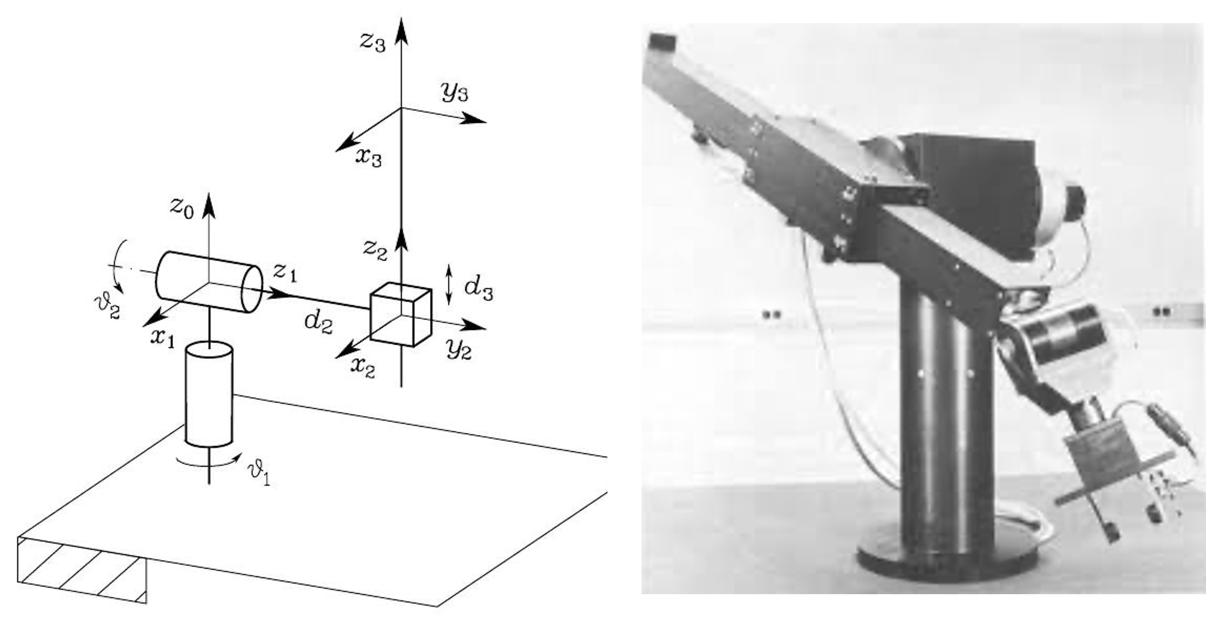
Two revolute joints plus one prismatic (\(\theta_1, \theta_2\) variable, \(d_3\) variable).
| Link | \(a_i\) | \(\alpha_i\) | \(d_i\) | \(\theta_i\) |
|---|---|---|---|---|
| 1 | \(0\) | \(-\pi/2\) | \(0\) | \(\theta_1^*\) |
| 2 | \(0\) | \(\pi/2\) | \(d_2\) | \(\theta_2^*\) |
| 3 | \(0\) | \(0\) | \(d_3^*\) | \(0\) |
Note that the rotation matrix of the end-effector depends only on the two revolute joints. The individual link matrices are
\[ \mathbf{A}^0_1 = \begin{bmatrix} c_1 & 0 & -s_1 & 0\\ s_1 & 0 & c_1 & 0\\ 0 & -1 & 0 & 0\\ 0 & 0 & 0 & 1 \end{bmatrix}, \quad \mathbf{A}^1_2 = \begin{bmatrix} c_2 & 0 & s_2 & 0\\ s_2 & 0 & -c_2 & 0\\ 0 & 1 & 0 & d_2\\ 0 & 0 & 0 & 1 \end{bmatrix}, \quad \mathbf{A}^2_3 = \begin{bmatrix} 1 & 0 & 0 & 0\\ 0 & 1 & 0 & 0\\ 0 & 0 & 1 & d_3\\ 0 & 0 & 0 & 1 \end{bmatrix}. \]
Their product gives the direct kinematics
\[ \mathbf{T}^0_3(\boldsymbol q) = \begin{bmatrix} c_1 c_2 & -s_1 & c_1 s_2 & c_1 s_2 d_3 - s_1 d_2\\ s_1 c_2 & c_1 & s_1 s_2 & s_1 s_2 d_3 + c_1 d_2\\ -s_2 & 0 & c_2 & c_2 d_3\\ 0 & 0 & 0 & 1 \end{bmatrix}, \qquad \boldsymbol q = \begin{bmatrix}\theta_1\\ \theta_2\\ d_3\end{bmatrix}. \]
3.3 Anthropomorphic arm (3R elbow)
Three revolute joints in the human-arm configuration: the first axis is perpendicular to the plane of the arm, the second and third axes are parallel to each other (the shoulder and elbow).
| Link | \(a_i\) | \(\alpha_i\) | \(d_i\) | \(\theta_i\) |
|---|---|---|---|---|
| 1 | \(0\) | \(\pi/2\) | \(0\) | \(\theta_1^*\) |
| 2 | \(a_2\) | \(0\) | \(0\) | \(\theta_2^*\) |
| 3 | \(a_3\) | \(0\) | \(0\) | \(\theta_3^*\) |
The individual link matrices are
\[ \mathbf{A}^0_1 = \begin{bmatrix} c_1 & 0 & s_1 & 0\\ s_1 & 0 & -c_1 & 0\\ 0 & 1 & 0 & 0\\ 0 & 0 & 0 & 1 \end{bmatrix}, \quad \mathbf{A}^1_2 = \begin{bmatrix} c_2 & -s_2 & 0 & a_2 c_2\\ s_2 & c_2 & 0 & a_2 s_2\\ 0 & 0 & 1 & 0\\ 0 & 0 & 0 & 1 \end{bmatrix}, \quad \mathbf{A}^2_3 = \begin{bmatrix} c_3 & -s_3 & 0 & a_3 c_3\\ s_3 & c_3 & 0 & a_3 s_3\\ 0 & 0 & 1 & 0\\ 0 & 0 & 0 & 1 \end{bmatrix}. \]
Their product gives the direct kinematics. Using \(c_{23}=\cos(\theta_2+\theta_3)\), \(s_{23}=\sin(\theta_2+\theta_3)\),
\[ \mathbf{T}^0_3(\boldsymbol q) = \begin{bmatrix} c_1 c_{23} & -c_1 s_{23} & s_1 & c_1(a_2 c_2 + a_3 c_{23})\\ s_1 c_{23} & -s_1 s_{23} & -c_1 & s_1(a_2 c_2 + a_3 c_{23})\\ s_{23} & c_{23} & 0 & a_2 s_2 + a_3 s_{23}\\ 0 & 0 & 0 & 1 \end{bmatrix}, \qquad \boldsymbol q = \begin{bmatrix}\theta_1\\ \theta_2\\ \theta_3\end{bmatrix}. \]
The end-effector frame does not coincide with frame 3 in general. A constant tool transform \(\mathbf{T}^3_e\) is appended to express the desired approach direction at the end-effector.
3.4 Spherical wrist (3R)
A spherical wrist is a three-revolute sub-chain whose three joint axes intersect at a common wrist centre point. Links are numbered from 4, since this sub-chain is typically mounted at the end of a 3R positioning arm (making a 6-DOF manipulator in total).
| Link | \(a_i\) | \(\alpha_i\) | \(d_i\) | \(\theta_i\) |
|---|---|---|---|---|
| 4 | \(0\) | \(-\pi/2\) | \(0\) | \(\theta_4^*\) |
| 5 | \(0\) | \(\pi/2\) | \(0\) | \(\theta_5^*\) |
| 6 | \(0\) | \(0\) | \(d_6\) | \(\theta_6^*\) |
The individual link matrices are
\[ \mathbf{A}^3_4 = \begin{bmatrix} c_4 & 0 & -s_4 & 0\\ s_4 & 0 & c_4 & 0\\ 0 & -1 & 0 & 0\\ 0 & 0 & 0 & 1 \end{bmatrix}, \quad \mathbf{A}^4_5 = \begin{bmatrix} c_5 & 0 & s_5 & 0\\ s_5 & 0 & -c_5 & 0\\ 0 & 1 & 0 & 0\\ 0 & 0 & 0 & 1 \end{bmatrix}, \quad \mathbf{A}^5_6 = \begin{bmatrix} c_6 & -s_6 & 0 & 0\\ s_6 & c_6 & 0 & 0\\ 0 & 0 & 1 & d_6\\ 0 & 0 & 0 & 1 \end{bmatrix}. \]
Their product gives the direct kinematics
\[ \mathbf{T}^3_6(\boldsymbol q) = \begin{bmatrix} c_4 c_5 c_6 - s_4 s_6 & -c_4 c_5 s_6 - s_4 c_6 & c_4 s_5 & c_4 s_5 d_6\\ s_4 c_5 c_6 + c_4 s_6 & -s_4 c_5 s_6 + c_4 c_6 & s_4 s_5 & s_4 s_5 d_6\\ -s_5 c_6 & s_5 s_6 & c_5 & c_5 d_6\\ 0 & 0 & 0 & 1 \end{bmatrix}, \qquad \boldsymbol q = \begin{bmatrix}\theta_4\\ \theta_5\\ \theta_6\end{bmatrix}. \]
The key property of the spherical wrist is that it produces a pure rotation: the wrist centre does not move as the wrist joints change, so position and orientation can be controlled independently. The resulting rotation matrix has exactly the form of the ZYZ Euler angle matrix \(\mathbf{R}_z(\varphi)\mathbf{R}_{y'}(\vartheta)\mathbf{R}_{z''}(\psi)\), where \(\varphi,\vartheta,\psi\) map to joints 4, 5, 6 respectively.
This decoupling is the basis of the arm-wrist decomposition for 6-DOF manipulators: the first three joints position the wrist centre (solved by inverse kinematics of the arm), and the last three joints orient the end-effector (solved by the ZYZ inverse formula). The end-effector frame coincides with frame 6 by convention for the spherical wrist.
More complex manipulators — such as a SCARA arm with a spherical wrist, or an anthropomorphic arm with an added wrist — can be assembled by concatenatingç their DH chains. The arm-wrist decomposition applies as long as the last three joint axes intersect at a single point.
4 Inverse kinematics
The inverse kinematics (IK) problem seeks joint variables that realise a desired pose:
\[ \boldsymbol q = h^{-1}(\boldsymbol x). \]
This is fundamentally harder than direct kinematics for several reasons:
- The equations are in general nonlinear, so closed-form solutions do not always exist.
- Multiple solutions typically exist (e.g. elbow-up vs. elbow-down).
- There may be infinitely many solutions for a kinematically redundant manipulator (\(n > m\)).
- There may be no solution if the desired pose lies outside the manipulator’s workspace.
4.1 Algebraic solution: planar 3R arm
For the planar 3R arm the task vector is
\[ \boldsymbol x = \begin{bmatrix} p_x \\ p_y \\ \varphi \end{bmatrix} = \begin{bmatrix} a_1 c_1 + a_2 c_{12} + a_3 c_{123}\\ a_1 s_1 + a_2 s_{12} + a_3 s_{123}\\ \theta_1 + \theta_2 + \theta_3 \end{bmatrix}. \]
Step 1. Remove the third link by computing the wrist point:
\[ p_{Wx} = p_x - a_3 c_\varphi, \qquad p_{Wy} = p_y - a_3 s_\varphi. \]
Step 2. Square and add to isolate \(\theta_2\):
\[ c_2 = \frac{p_{Wx}^2 + p_{Wy}^2 - a_1^2 - a_2^2}{2a_1 a_2}, \quad -1 \le c_2 \le 1, \] \[ s_2 = \pm\sqrt{1-c_2^2}, \qquad \boxed{\;\theta_2 = \operatorname{atan2}(s_2,c_2)\;}\tag{IK.1} \]
The two signs give elbow-up (\(s_2>0\)) and elbow-down (\(s_2<0\)) configurations.
Step 3. With \(\theta_2\) known, solve a linear system for \(\theta_1\):
\[ s_1 = \frac{(a_1 + a_2 c_2)\,p_{Wy} - a_2 s_2\,p_{Wx}}{p_{Wx}^2 + p_{Wy}^2}, \qquad c_1 = \frac{(a_1 + a_2 c_2)\,p_{Wx} + a_2 s_2\,p_{Wy}}{p_{Wx}^2 + p_{Wy}^2}, \] \[ \boxed{\;\theta_1 = \operatorname{atan2}(s_1, c_1)\;}\tag{IK.2} \]
Step 4. The orientation equation closes the chain:
\[ \boxed{\;\theta_3 = \varphi - \theta_1 - \theta_2\;}\tag{IK.3} \]
4.2 Geometric solution: planar 3R arm
The same result follows from triangle geometry. The law of cosines on the triangle formed by the two links and the wrist point gives:
\[ c_2 = \frac{p_{Wx}^2 + p_{Wy}^2 - a_1^2 - a_2^2}{2a_1 a_2}, \qquad \theta_2 = \pm\cos^{-1}(c_2).\tag{IK.1} \]
Introducing the auxiliary angles
\[ \alpha = \operatorname{atan2}(p_{Wy}, p_{Wx}), \qquad \beta = \cos^{-1}\!\left( \frac{p_{Wx}^2 + p_{Wy}^2 + a_1^2 - a_2^2}{2a_1\sqrt{p_{Wx}^2 + p_{Wy}^2}}\right), \]
the base joint is
\[ \boxed{\;\theta_1 = \alpha \mp \beta\;}\tag{IK.2} \]
with the sign matched to the elbow choice, and
\[ \boxed{\;\theta_3 = \varphi - \theta_2 - \theta_1\;}\tag{IK.3} \]
4.3 Inverse kinematics of the spherical wrist
For a manipulator with a spherical wrist, the IK decouples:
- Arm IK: compute the wrist centre position from the desired end-effector pose and tool length; solve the arm’s IK for the first three joints.
- Wrist IK: extract the desired wrist rotation \(\mathbf{R}_{\text{wrist}}\) and solve the ZYZ inverse problem for joints 4, 5, 6.
This decoupling is possible only because the spherical wrist axes intersect, so changing wrist joints does not move the wrist centre.